
提到Tidymodels包前,先认识一个人-Hadley Wickham是《R for Data Science》的合著者,也是RStudio的首席科学家。在Tidy Tools中,他为处理数据的计算机接口提出了四条基本原则:
- Reuse existing data structures.
- Compose simple functions with the pipe.
- Embrace functional programming.
- Design for humans.
这些原则在他的R包 tidyverse中实现,Tidymodels也遵循相同的思想设计,旨在为机器学习提供一个便捷的平台。
根据官方的一个case,我们来尝试下 Tidymodels 的优势和建模思想:
示例数据:
# 需要安装glmnet, ranger, readr, tidymodels, 和 vip包
# install.packages("tidymodels")

library(tidymodels)
library(readr)       # 导入数据
library(vip)         # 变量重要程度

# 绘图
library(ggplot2)
library(ggthemes)
1)读取数据
# 检测电脑CPU
cores <- parallel::detectCores()
cores

# 读取演示数据
hotels <-
  read_csv('hotels.csv') %>%
  mutate_if(is.character, as.factor)

dim(hotels)
2)逻辑回归建模workflow
# 我们将建立一个模型来预测实际入住的酒店哪些包括儿童/婴儿,哪些没有。
# 结果变量儿童是一个有两个层次的因素变量(children和none)
# 不均衡样本可以用themis包(tidymodels生态系统包)来估算样本使其均衡。
# 逻辑回归
# 创建训练集和测试集
set.seed(123)
splits <- initial_split(hotels, strata = children)
hotel_other <- training(splits)
hotel_test <- testing(splits)
# 查看训集中children的比例
hotel_other %>%
count(children) %>%
mutate(prop = n / sum(n))
#> # A tibble: 2 x 3
#> children n prop
#> <fct> <int> <dbl>
#> 1 children 3048 0.0813
#> 2 none 34452 0.919
# 查看测试集中children的比例
hotel_test %>%
count(children) %>%
mutate(prop = n / sum(n))
#> # A tibble: 2 x 3
#> children n prop
#> <fct> <int> <dbl>
#> 1 children 990 0.0792
#> 2 none 11510 0.921
# 拆分验证集
set.seed(234)
val_set <- validation_split(hotel_other,
strata = children,
prop = 0.80)
val_set
#> # Validation Set Split (0.8/0.2) using stratification
#> # A tibble: 1 x 2
#> splits id
#> <named list> <chr>
#> 1 <split [30K/7.5K]> validation
# 逻辑回归建模
lr_mod <-
logistic_reg(penalty = tune(), mixture = 1) %>%
set_engine("glmnet", num.threads = cores)
# 节假日管理
holidays <- c(
"AllSouls",
"AshWednesday",
"ChristmasEve",
"Easter",
"ChristmasDay",
"GoodFriday",
"NewYearsDay",
"PalmSunday"
)
# 建模workflow
lr_recipe <-
recipe(children ~ ., data = hotel_other) %>%
step_date(arrival_date) %>%
step_holiday(arrival_date, holidays = holidays) %>%
step_rm(arrival_date) %>%
step_dummy(all_nominal(),-all_outcomes()) %>%
step_zv(all_predictors()) %>%
step_normalize(all_predictors())
# 建模
lr_workflow <-
workflow() %>%
add_model(lr_mod) %>%
add_recipe(lr_recipe)
# 惩罚因子参数
lr_reg_grid <- tibble(penalty = 10 ^ seq(-4,-1, length.out = 30))
lr_reg_grid %>% top_n(-5) # lowest penalty values
#> Selecting by penalty
#> # A tibble: 5 x 1
#> penalty
#> <dbl>
#> 1 0.0001
#> 2 0.000127
#> 3 0.000161
#> 4 0.000204
#> 5 0.000259
lr_reg_grid %>% top_n(5) # highest penalty values
#> Selecting by penalty
#> # A tibble: 5 x 1
#> penalty
#> <dbl>
#> 1 0.0386
#> 2 0.0489
#> 3 0.0621
#> 4 0.0788
#> 5 0.1
# 运行模型自动调参
lr_res <-
lr_workflow %>%
tune_grid(
val_set,
grid = lr_reg_grid,
control = control_grid(save_pred = TRUE),
metrics = metric_set(roc_auc)
)
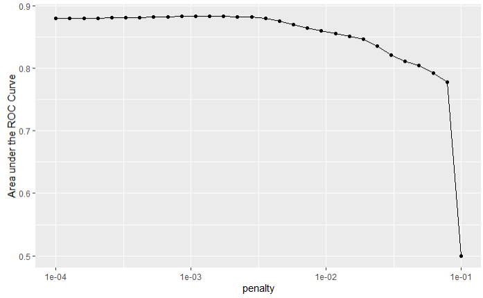
# 绘制惩罚因子和AUC曲线
lr_res %>%
collect_metrics() %>%
ggplot(aes(x = penalty, y = mean)) +
geom_point() +
geom_line() +
ylab("Area under the ROC Curve") +
scale_x_log10()
# 打印前15模型
top_models <-
lr_res %>%
show_best("roc_auc", n = 15) %>%
arrange(penalty)
top_models
# 选择最佳模型
lr_best <-
lr_res %>%
collect_metrics() %>%
arrange(penalty) %>%
slice(12)
lr_best
#> # A tibble: 1 x 6
#> penalty .metric .estimator mean n std_err
#> <dbl> <chr> <chr> <dbl> <int> <dbl>
#> 1 0.00137 roc_auc binary 0.881 1 NA
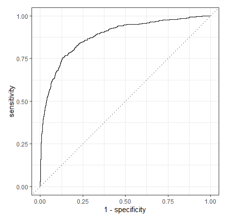
# 绘制ROC曲线
lr_auc <-
lr_res %>%
collect_predictions(parameters = lr_best) %>%
roc_curve(children, .pred_children) %>%
mutate(model = "Logistic Regression")
autoplot(lr_auc)
建模过程及ROC曲线:
3)随机森林建模
# 随机森林
rf_mod <-
rand_forest(mtry = tune(),
min_n = tune(),
trees = 1000) %>%
set_engine("ranger", num.threads = cores) %>%
set_mode("classification")
# 构建workflow
rf_recipe <-
recipe(children ~ ., data = hotel_other) %>%
step_date(arrival_date) %>%
step_holiday(arrival_date) %>%
step_rm(arrival_date)
rf_workflow <-
workflow() %>%
add_model(rf_mod) %>%
add_recipe(rf_recipe)
# 查看信息
rf_mod
#> Random Forest Model Specification (classification)
#>
#> Main Arguments:
#> mtry = tune()
#> trees = 1000
#> min_n = tune()
#>
#> Engine-Specific Arguments:
#> num.threads = cores
#>
#> Computational engine: ranger
# show what will be tuned
rf_mod %>%
parameters()
#> Collection of 2 parameters for tuning
#>
#> id parameter type object class
#> mtry mtry nparam[?]
#> min_n min_n nparam[+]
#>
#> Model parameters needing finalization:
#> # Randomly Selected Predictors ('mtry')
#>
#> See `?dials::finalize` or `?dials::update.parameters` for more information.
# 运行随机森林建模
set.seed(345)
rf_res <-
rf_workflow %>%
tune_grid(
val_set,
grid = 25,
control = control_grid(save_pred = TRUE),
metrics = metric_set(roc_auc)
)
#> i Creating pre-processing data to finalize unknown parameter: mtry
# 显示最佳建模模型信息
rf_res %>%
show_best(metric = "roc_auc")
#> # A tibble: 5 x 7
#> mtry min_n .metric .estimator mean n std_err
#> <int> <int> <chr> <chr> <dbl> <int> <dbl>
#> 1 8 7 roc_auc binary 0.933 1 NA
#> 2 6 18 roc_auc binary 0.933 1 NA
#> 3 9 12 roc_auc binary 0.932 1 NA
#> 4 3 3 roc_auc binary 0.932 1 NA
#> 5 5 35 roc_auc binary 0.932 1 NA
# 绘制随机森林调参ROC趋势
autoplot(rf_res)
# 最佳参数
rf_best <-
rf_res %>%
select_best(metric = "roc_auc")
rf_best
#> # A tibble: 1 x 2
#> mtry min_n
#> <int> <int>
#> 1 8 7
rf_res %>%
collect_predictions()
#> # A tibble: 187,475 x 7
#> id .pred_children .pred_none .row mtry min_n children
#> <chr> <dbl> <dbl> <int> <int> <int> <fct>
#> 1 validation 0.00158 0.998 11 12 7 none
#> 2 validation 0.000167 1.00 13 12 7 none
#> 3 validation 0.000286 1.00 31 12 7 none
#> 4 validation 0.000168 1.00 32 12 7 none
#> 5 validation 0.00075 0.999 36 12 7 none
#> # … with 1.875e+05 more rows
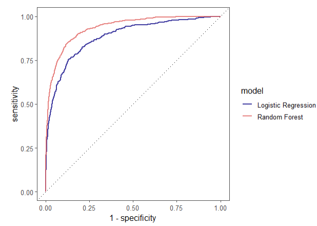
# 绘制ROC曲线(逻辑回归和随机森林)
rf_auc <-
rf_res %>%
collect_predictions(parameters = rf_best) %>%
roc_curve(children, .pred_children) %>%
mutate(model = "Random Forest")
bind_rows(rf_auc, lr_auc) %>%
ggplot(aes(
x = 1 - specificity,
y = sensitivity,
col = model
)) +
theme_few() +
geom_path(lwd = 0.8, alpha = 0.8) +
geom_abline(lty = 3) +
coord_equal() +
scale_color_viridis_d(option = "plasma", end = .6)
# 提取最佳模型
last_rf_mod <-
rand_forest(mtry = 8,
min_n = 7,
trees = 1000) %>%
set_engine("ranger", num.threads = cores, importance = "impurity") %>%
set_mode("classification")
# 运行
last_rf_workflow <-
rf_workflow %>%
update_model(last_rf_mod)
# 建模
set.seed(345)
last_rf_fit <-
last_rf_workflow %>%
last_fit(splits)
last_rf_fit
#> # Monte Carlo cross-validation (0.75/0.25) with 1 resamples
#> # A tibble: 1 x 6
#> splits id .metrics .notes .predictions .workflow
#> * <list> <chr> <list> <list> <list> <list>
#> 1 <split [37.5K… train/test… <tibble [2 … <tibble [0… <tibble [12,500… <workflo…
last_rf_fit %>%
collect_metrics()
#> # A tibble: 2 x 3
#> .metric .estimator .estimate
#> <chr> <chr> <dbl>
#> 1 accuracy binary 0.947
#> 2 roc_auc binary 0.922
# 提取重要变量,此处我们选取Top20
last_rf_fit %>%
pluck(".workflow", 1) %>%
pull_workflow_fit() %>%
vip(num_features = 20)
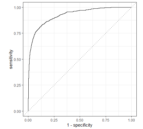
# 绘制ROC曲线
last_rf_fit %>%
collect_predictions() %>%
roc_curve(children, .pred_children) %>%
autoplot()建模过程及ROC曲线:

总体来说,框架设计非常便捷,建模过程和选参过程很智能,有点像keras的风格。
参考资料:
1.https://www.r-bloggers.com/welcome-to-the-tidyverse/
2.https://www.tidymodels.org/start/case-study/
